---
title: "Getting Started"
output:
rmarkdown::html_vignette:
toc: true
vignette: >
%\VignetteIndexEntry{Getting Started}
%\VignetteEngine{knitr::rmarkdown}
%\VignetteEncoding{UTF-8}
---
```{r, include = FALSE, message=FALSE, results='hide'}
knitr::opts_chunk$set(
collapse = TRUE,
comment = "#>",
eval = FALSE
)
library(threeBrain)
```
`threeBrain` is an R package that renders `FreeSurfer` or `AFNI/SUMA` files in the modern web browsers. The goal is to provide 3D viewers that are **powerful**, **interactive**, **easy-to-share**.
## Directory Setup
The basic setup of a typical subject folder should look like this:
```
Project Directory
└─Subject code
├─mri - Atlas, T1 and/or CT image files (*.mgz, transforms, ...)
├─surf - FreeSurfer surface files (pial, sulc, ...)
├─SUMA - (Optional) SUMA standard 141 surfaces (std.141.*)
└─... - Other files
```
If you are using `FreeSurfer` to generate MRI reconstruction, then you are all set! For `AFNI/SUMA` users, please place your `SUMA` folder under subject folder.
If you don't have any `FreeSurfer` folders, you can download a sample archive from [here](https://github.com/dipterix/threeBrain-sample/releases), choose `N27-complete.zip`, and extract to your download directory. Once extracted, you will have a `N27` subject folder in the `~/Downloads/` directory. The directory tree looks exactly the same as described above.
In the following context, I will use `~/Downloads/N27` as an example
## Generate Viewer Object
```{r setup, eval=FALSE}
library(threeBrain)
subject_code <- "N27"
subject_path <- "~/Downloads/N27"
brain <- threeBrain(subject_path, subject_code)
print(brain)
#> Subject - N27
#> Transforms:
#>
#> - FreeSurfer TalXFM [from scanner to MNI305]:
#> [,1] [,2] [,3] [,4]
#> [1,] 0.9692 -0.0029 -0.0134 -0.1638
#> [2,] 0.0062 0.9685 0.0492 -2.0717
#> [3,] 0.0145 0.0276 0.9541 0.1361
#> [4,] 0.0000 0.0000 0.0000 1.0000
#>
#> - Torig [Voxel CRS to FreeSurfer origin, vox2ras-tkr]
#> [,1] [,2] [,3] [,4]
#> [1,] -1 0 0 128
#> [2,] 0 0 1 -128
#> [3,] 0 -1 0 128
#> [4,] 0 0 0 1
#>
#> - Norig [Voxel CRS to Scanner center, vox2ras]
#> [,1] [,2] [,3] [,4]
#> [1,] -1 0 0 128.5
#> [2,] 0 0 1 -145.5
#> [3,] 0 -1 0 146.5
#> [4,] 0 0 0 1.0
#>
#> - Scanner center relative to FreeSurfer origin
#> [1] -0.5 17.5 -18.5
#>
#> - FreeSurfer RAS to MNI305, vox2vox-MNI305
#> [,1] [,2] [,3] [,4]
#> [1,] 0.9692 -0.0029 -0.0134 0.12365
#> [2,] 0.0062 0.9685 0.0492 -18.10715
#> [3,] 0.0145 0.0276 0.9541 17.31120
#> [4,] 0.0000 0.0000 0.0000 1.00000
#> Surface information (total count 1)
#> Loading required namespace: rstudioapi
#> pial [ std.141 ]
#> Volume information (total count 1)
#> T1
```
If this is the first time, it might take a while to import and generate cache files.
## Visualization
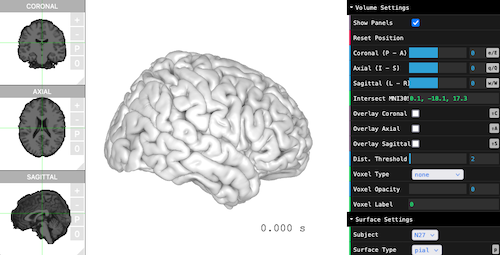
Visualizing the viewer is simply just one line.
```{r, eval=FALSE}
brain$plot()
```
 ## Surface, Volume, Atlas
By default, the viewers only load the following information. Only the `pial` surfaces are mandatory, other files are optional.
* T1 (MR images) and transforms (optional)
- `mri/brain.finalsurfs.mgz`
- `mri/transforms/talairach.xfm`
* `pial` (mandatory) and `sulc` (optional)
- `surf/*h.pial` or `SUMA/std.141.*h.pial[.asc|gii]`
- `surf/*h.sulc` or `SUMA/std.141.*h.sulc.1D`
* `aparc+aseg` (optional)
- `mri/aparc+aseg.mgz`
The T1 image is automatically detected if `brain.finalsurfs.mgz` is missing. The following alternatives are `brainmask.mgz`, `brainmask.auto.mgz`, `T1.mgz`.
To load more than one surfaces, please specify the surface types when loading the viewer. The available surface types are:
* `pial` - (default)
* `smoothwm`, `white` - (smoothed) white matter
* `inflated`, `sphere` - inflated surfaces
* `pial-outer-smoothed` - ('FreeSurfer'-only) smoothed surface tightly wrapping the pial surface
* `inf_200` - ('SUMA'-only) inflated pial surface
The atlas type can be selected from `aparc+aseg`, `aparc.a2009s+aseg`, `aparc.DKTatlas+aseg`, or `aseg`. To load a specific atlas, please make sure the corresponding file exists in `mri/`. For example, `mri/aseg.mgz`.
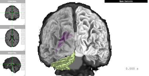
The following example loads `pial` and `smoothwm`, with `aseg` as atlas. The viewer shows 'Coronal' plane, smoothed white matter, 'Ventricle', and 'Cerebellum' all together in one scene.
```{r, eval=FALSE}
brain <- threeBrain(
subject_path, subject_code,
surface_types = c('pial', 'smoothwm'),
atlas_types = 'aseg')
brain$plot(
controllers = list(
"Voxel Type" = "aseg",
"Voxel Label" = "4,5,6,7",
"Surface Type" = "smoothwm",
"Left Opacity" = 0.4,
"Overlay Coronal" = TRUE
),
control_display = FALSE,
camera_pos = c(0, -500, 0)
)
```
## Surface, Volume, Atlas
By default, the viewers only load the following information. Only the `pial` surfaces are mandatory, other files are optional.
* T1 (MR images) and transforms (optional)
- `mri/brain.finalsurfs.mgz`
- `mri/transforms/talairach.xfm`
* `pial` (mandatory) and `sulc` (optional)
- `surf/*h.pial` or `SUMA/std.141.*h.pial[.asc|gii]`
- `surf/*h.sulc` or `SUMA/std.141.*h.sulc.1D`
* `aparc+aseg` (optional)
- `mri/aparc+aseg.mgz`
The T1 image is automatically detected if `brain.finalsurfs.mgz` is missing. The following alternatives are `brainmask.mgz`, `brainmask.auto.mgz`, `T1.mgz`.
To load more than one surfaces, please specify the surface types when loading the viewer. The available surface types are:
* `pial` - (default)
* `smoothwm`, `white` - (smoothed) white matter
* `inflated`, `sphere` - inflated surfaces
* `pial-outer-smoothed` - ('FreeSurfer'-only) smoothed surface tightly wrapping the pial surface
* `inf_200` - ('SUMA'-only) inflated pial surface
The atlas type can be selected from `aparc+aseg`, `aparc.a2009s+aseg`, `aparc.DKTatlas+aseg`, or `aseg`. To load a specific atlas, please make sure the corresponding file exists in `mri/`. For example, `mri/aseg.mgz`.
The following example loads `pial` and `smoothwm`, with `aseg` as atlas. The viewer shows 'Coronal' plane, smoothed white matter, 'Ventricle', and 'Cerebellum' all together in one scene.
```{r, eval=FALSE}
brain <- threeBrain(
subject_path, subject_code,
surface_types = c('pial', 'smoothwm'),
atlas_types = 'aseg')
brain$plot(
controllers = list(
"Voxel Type" = "aseg",
"Voxel Label" = "4,5,6,7",
"Surface Type" = "smoothwm",
"Left Opacity" = 0.4,
"Overlay Coronal" = TRUE
),
control_display = FALSE,
camera_pos = c(0, -500, 0)
)
```